Revisiting Hachure Lines: Dynamic Hachure Contours in ArcGIS Pro
- Warren
- Aug 13, 2020
- 10 min read

Updated: Jan 3, 2024
Hachure lines have been on my cartographic to-do list for a very long time. The craftsmanship in the hand-drawn details of historical maps is just one of the many things that pulled me into geography, cartography, and maps in general in the first place. Trying to find ways to bring some ounce of those techniques into the digital maps I create has inspired a number of cartographic experiments.

This installment is by no means the first. This particular venture into hachure terrain depiction follows several previous attempts and builds on the work of others, specifically the concepts/methods here and here.
Just a word of warning before we dive in: the methodology I developed below is for ArcGIS Pro, and some steps require the Spatial Analyst extension. The steps which require the extension are optional but I found that they significantly improve the results through the generalization of the intermediate raster datasets. As well, the concept isn't new and, as mentioned, builds on the steps outlined here.
Methodology
Now that all that's out of the way, let's dive into the methodology and start shading some terrain. The loose process is as follows:
Grab a DEM from your favourite source.
Smooth it out with some Focal Statistics.
Create Slope and Aspect Rasters.
Reclassify these rasters.
Generalize and refine the rasters.
Convert the raster to polygons.
Union these polygons.
Intersect these polygons with contour lines.
Render contours with Arcade Expressions.
For all the raster-slinging details, keep reading!
DEM
The starting point is a DEM covering your area of interest. Do yourself a favour, and be sure to extract or clip your DEM to your specific area of interest. This will have implications when we go to create our slope raster.
The next step is to smooth this DEM raster to some degree. I don't have any prescribed values here, but I typically used the Focal Statistics to perform a Mean operation for a 10-cell neighbourhood (you can also use raster functions if you don't have the license level for this tool). This will vary with your DEM resolution, so feel free to experiment (you may have to run through the process a few times). Ultimately, by smoothing our DEM, we'll ensure that our following Slope and Aspect rasters are also slightly smoothed and will serve to minimize the fragmentation of our final result.
At this point, since I was testing the methods on various locations, I also generated contours from my smoothed DEM rather than hunting down some open data source for contour lines in my test locations. Conveniently, these contours were also nice and smooth. I generated these contours in the same spatial unit as the raster and at 1 unit intervals. Once created, I also took a moment to add a text field to contain the contour elevation. I named this field ELEVATION. This field would help simplify some of the Arcade Expressions later on. I used a few queries like WHERE ELEVATION LIKE '%0' OR ELEVATION LIKE '%5' to select contours with either 10 or 5 unit intervals.

Slope and Aspect Rasters
Using the newly smoothed DEM as an input, create a Slope and Aspect raster. Again, these can be created using geoprocessing tools (slope/aspect) or the appropriate Raster Functions (slope/aspect - wait, there's a Slope-Aspect function?!). It's self-explanatory, but these rasters describe specific aspects (see what I did there?) of the terrain and form the primary criteria that we'll use moving forward to control the rendering of our hachure lines. For convenience, from here on out, I'll simply refer to these rasters collectively as 'terrain rasters'. The majority of the process is done in parallel to both rasters now.


Reclassification of Terrain Rasters
The next step is to take our terrain rasters and reclassify their cells into a series of discrete values using the Reclassify Tool. This allows us to group cell values together into easily processed chunks.
Aspect
The aspect raster is fairly straightforward, and the reclassified values are broken into classifications based on the directionality of the terrain. Through some experimentation, I found that splitting the aspect values into 60-degree segments worked well. I assigned these segments a value from 1 to 7 based on their 'shaded-ness'.


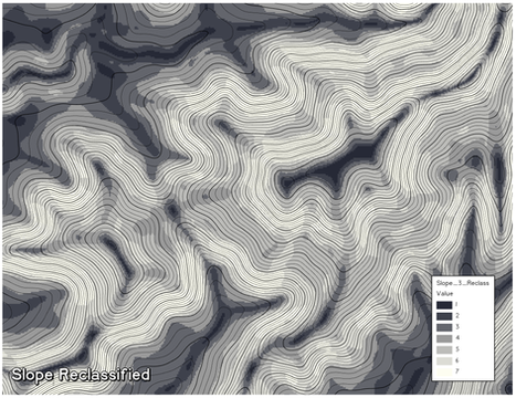
Slope
Reclassification of the slope raster is a little more subjective. I opted not to hardcode any specific thresholds in favour of allowing some experimentation and leaving room for artistic representation of the terrain.
Through my testing, I found that a quick and easy route was to first apply a Classified Symbology to the Slope raster with 7 classes and Natural Breaks (Jenks) class breaks. This quickly showed me where clusters of slope values existed. This was why it was important to clip your DEM to the extent you plan on mapping; a mountain or canyon included in your DEM but out of frame would impact the class breaks and make the rest of the process difficult. From here, you can tweak the class breaks as required, ensuring that your areas of visual interest land in the higher classes.


Generalization of Terrain Rasters
The following steps are now all conducted separately but in parallel for both the slope and aspect rasters. These steps also require the Spatial Analyst extension but are optional, as mentioned, although highly recommended. These steps generalize the terrain rasters and significantly reduce the fragmentation of the results (shown below).
At this point, I don't know of any alternatives off the top of my head, so if you don't have a Spatial Analyst extension, skip ahead to the Convert to Polygon step.
The methodology I followed leans heavily on this process for the generalization of classified imagery, which is described in detail here. I simply modify a few parameters when running the tools described so the 'step-by-step' gets a little more brief in the following descriptions.
Majority Filter: removes single cells within the terrain rasters that don't match their neighbours.
Boundary Clean: Smoothes the boundary between the classified zones within our terrain rasters. I ran this with the SORT_TYPE = DESCEND meaning that smaller groupings will be consumed by larger regions. We ultimately want to remove small clusters of cells, they won't have a significant impact on our hachure renderings. I also opted to use the default and run the EXPAND-SHRINK process twice.
Region Group: Takes like clusters of cells and essentially assigns them an ID and a LINK back to the original cell value. Useful for quantifying clusters of cell values for the next step. I ran this with the NUMBER_NEIGHBOURS set to 4. I didn't want cells that were diagonal to be considered part of the same region, I wanted to mitigate those loose neighbour connections.
Extract By Attribute: This tool omits regions from our Region Group raster that don't meet a specified criteria. This step is also a little subjective. I found it helpful to pan through your Region Group raster at a scale that was close to what you planned on mapping. While panning identify those clusters that look just a little too small to really impact the overall aesthetic of your map; note their CELL COUNT attributes. Use this cell count value and create an extraction expression to select all regions where the "CELL_COUNT >= some threshold". This will create a raster with NO DATA value holes where those small regions were omitted.
Nibble: The Nibble tool takes the raster output from your Boundary Clean tool as an input and the raster from the Extract by Attribute output as a mask. This will fill those holes in the terrain raster with valid values and minimize the small clusters.
Convert Terrain Rasters to Polygons
Now that our rasters have been generalized, we can convert them to polygons using the Raster to Polygon tool. Now we're done tossing raster cells around, and we're working with vector data again. Once these polygons are converted, I recommend renaming their GRIDCODE fields to something more logical Might I suggest SLOPE and ASPECT (*these are the names I anticipate in the Arcade expressions later on but they can be configured to your liking).

Union Terrain Polygons
Hold on tight, there are only a few more progress bars to watch patiently! Now that we have a polygon for each terrain variable, we'll Union these polygons to generate a dataset where each feature in the output has a homogeneous combination of the Slope and Aspect.

Intersect with Contours
The final processing step is to intersect these mega terrain variable polygons with our contour lines, making them 'aware' of the terrain conditions they cross. Confirm that the output geometry is set to Line, and proceed to watch the final progress bar!
You made it this far?! still reading?
GOOD!
Because the next part was worth the wait!
Attribute-Driven Symbology
Admittedly, I've only just begun to realize the potential of using Arcade Expressions in ArcGIS Pro. I've used them to quickly concatenate address strings with conditional logic and colour code curling rock map symbols, but they're capable of so much more. In fact, there are plenty of other great reasons to use them, but let's just quietly put Rendering Hachure Lines at the top of that list.
To use the Arcade Expressions to control the rendering of hachure marks, we'll enable the symbol property connections to allow for attribute-driven symbology.

What we're looking to do is use the terrain attributes we derived from our rasters and transfer them to our contours to drive the symbology of our contour lines that approximate, as well as possible, the hachure lines we're seeking. I've grouped this symbology into four main variables discussed below:
Contour Stroke Weight
Hachure Stroke Weight
Hachure Band Width
Hachure Stroke Density
Each of the expressions that control these symbol variables is configurable, and tweaking the HACHURE CONSTRAINTS variables in the expressions will change how the symbols are rendered. Remember that it's highly recommended you determine a scale for your map and set it as a reference scale. Once you've set the scale, experiment with these constraint variables until you achieve the desired effect.

Contour Stroke Weight
One interesting fact is I actually started this symbology portion of the process with the humble Railroad symbol. Shoutout to the default symbol gallery! Obviously, I then modified and refined the symbol for my purposes and saved a style file so you don't have to start from scratch like me.

The Contour Stroke Weight expression serves to vary the weight of the contour line itself. This expression is actually optional, and you can remove or turn off the contour lines depending on what you're trying to achieve with your map. If you're really adventurous, you could remove the hachure strokes altogether and apply some of those expressions to the stroke weight of the contours (wink, wink).
// OVERVIEW
// Increase width of contour line for 100ft increments
// elevation variable
var elev = $feature.ELEVATION

// if ends in '00' we'll increase the width otherwise use default of 0.25. Everything else will be a hidden contour and will only have hachures.
var width = When(Right(elev,2) == '00', 0.5, Right(elev,2) == '25', 0.25, Right(elev,2) == '50', 0.25, Right(elev,2) == '75', 0.25, 0)

return width
Hachure Stroke Weight (Shape Line Symbol - Line Width)
This expression controls the weight of the Hachure stroke. Where the terrain is steep and the aspect is facing Southeast, weight will be heavier. The inverse will be true where the slope is shallow, and the terrain faces Northwest.
// OVERVIEW
// increase the stroke weight of hachure ticks based on the aspect/slope
// create some terrain constaints
// these lower constraints will prevent anything less from rendering

// SLOPE
var slope_min = 3
var slope_max = 7

// ASPECT
var aspect_min = 3
var aspect_max = 7

// since we've constrained our inputs to a subset of our original 7 reclassifications, we'll scale these variables back to a range of 7 (0-7)
var slope = (($feature.SLOPE - slope_min) * 7) / (slope_max - slope_min) + 0
var aspect = (($feature.ASPECT - aspect_min) * 7) / (aspect_max - aspect_min) + 0

// TERRAIN
var terrain = (slope + aspect)
var terrain_min = 0
var terrain_max = 14
var terrain_range = terrain_max - terrain_min // anticipated terrain scale

// HACHURE WEIGHT CONSTRAINTS
// these values will constrain the weight of hachure marks along the contours

var width_min = 0.1
var width_max = 2
var width_range = width_max - width_min

// TERRAIN ENCODING
var hachure_weight = (((terrain - terrain_min) * width_range) / terrain_max) + width_min

// RETURN STROKE WEIGHT
return IIf($feature.ASPECT > aspect_min && $feature.SLOPE > slope_min, Text(hachure_weight), width_min)
Hachure Band Width (Shape Line Symbol - Size)
This expression controls the width of the hachure 'band' (the length of the individual hachure strokes). Where the terrain is mild, the band will be wider to close the gap between contour lines. Where the terrain is intense, the band width should be narrowed to prevent overlaps and any negative visual effects.
// stretch the width of the 'hachure band' based on the slope
// in high slope areas the hachure strokes will be short to accomodate clustered contours
// in low slope areas the strokes will be lengthened to cover more of the slope
// create some terrain constaints
// we'll use these constraints to render only those contours that exceed these conditions

// SLOPE
var slope_min = 3
var slope_max = 7
// ASPECT
var aspect_min = 3
var aspect_max = 7

// since we've constrained our inputs to a subset of our original 7 reclassifications, we'll scale these variables back to a range of 7 (0 -7)

var slope = (($feature.SLOPE - slope_min) * 7) / (slope_max - slope_min) + 0
var aspect = (($feature.ASPECT - aspect_min) * 7) / (aspect_max - aspect_min) + 0

// TERRAIN
// here we'll map the anticipated values from the terrain inputs above to a easy to use 'terrain variable'
var terrain = (slope + aspect)
var terrain_min = 0
var terrain_max = 14
var terrain_range = terrain_max - terrain_min // 14 anticipated terrain scale

// HACHURE CONSTRAINTS
// create some hachure band constraints
// these values will dictate the min and max widths of the hachure band
var size_min = 1
var size_max = 4
var size_range = size_max - size_min

// TERRAIN ENCODING
// map the slope values to a hachure band width
var hachure_size = (((terrain - terrain_min) * size_range) / terrain_range) + size_min

// INVERT VALUE
// here we invert the size value (steep slope = narrow, shallow slope = wide)
return IIf($feature.ASPECT > aspect_min && $feature.SLOPE > slope_min, Text((Abs(hachure_size - size_max) + size_min)), 0)
Hachure Stroke Density (Marker Placement Properties)
This expression controls the placement property of the hachure tick mark. Where the terrain is more 'intense,' the placement will be closer together. The inverse will be true when the terrain is gentle.
// OVERVIEW
// densify the placement of hachure ticks based on the aspect/slope
// create some terrain constaints
// these lower constraints will prevent anything less from rendering

// SLOPE
var slope_min = 3
var slope_max = 7

// ASPECT
var aspect_min = 3
var aspect_max = 7

// since we've constrained our inputs to a subset of our original 7 reclassifications, we'll scale these variables back to a range of 7 (0-7)

var slope = (($feature.SLOPE - slope_min) * 7) / (slope_max - slope_min) + 0
var aspect = (($feature.ASPECT - aspect_min) * 7) / (aspect_max - aspect_min) + 0

// TERRAIN
var terrain = (slope + aspect)
var terrain_min = 0
var terrain_max = 14
var terrain_range = terrain_max - terrain_min // anticipated terrain scale

// HACHURE DENSITY CONSTRAINTS
// these values will constrain the placement of hachure marks along the contours
var dense_min = 0.5
var dense_max = 4
var dense_range = dense_max - dense_min

// TERRAIN ENCODING
var hachure_density = (((terrain - terrain_min) * dense_range) / terrain_max) + dense_min

// INVERT
// Invert the density value obtained so it logically scales with the shading behaviour we'd expect
return IIf($feature.ASPECT > aspect_min && $feature.SLOPE > slope_min, Text((Round(Abs(hachure_density - dense_max) + dense_min, 2))), 0)
Examples & Final Thoughts
This method is still a work in progress, and I'm continuing to experiment with refining it, but I thought it was worth sharing, and others can also experiment! Here are some maps I've been testing; you'll notice many are attempting to achieve that visual aesthetic of the Chevalier map.
If you try it out, I'd love to see your maps! Send me your maps @WarrenDz.


Hi Warren, great walk over the various steps to reach to that look! By any chance, have you cover Erwin Raisz's landform style where he shades with Hachures on the sides with others having a solid black? Thanks!
This technique applied with a semi-transparent slope raster on top of the generalized aspect polygons.